4 Coding
4.1 MATLAB (Release 2/2016)
Encountered in: MAT_SCI 405, 408
MATLAB is a powerful computing environment that is commonly used by scientists and engineers of all disciplines for numerical simulation, data analysis, data visualization, hardware control, and creation of custom graphical user interfaces.
MATLAB’s built-in functional utility is vast, and this is further supported by an active user community that interacts at the MathWorks File Exchange. There, you can find free user-generated content — functions, applictions, examples, drivers, etc, that may prove useful in your coursework and research.
MATLAB is installed on the computers in the Bodeen Laboratory and is also available for purchase by students ($72/yr on campus, including VPN; $130 off campus). Many research groups also have license subscriptions that can be utilized for your academic projects.
Below is a basic introduction to working with MATLAB. Some good resources and tutorials are linked below for further investigation.
Suggested Resources:
Introduction to MATLAB, David Houcque, Northwestern University (2005) eReserve Link4
Ilya Mikhelson (Northwestern EECS) has developed a series of MATLAB tutorials and posted them on YouTube. Specifically useful tutorials are following
4.1.1 Interfacing with MATLAB
When a user first opens MATLAB (this guide is written for the current version of MATLAB as of 2/2017: MATLAB 9.1) as shown in Fig. 1 with various sub-windows visible.
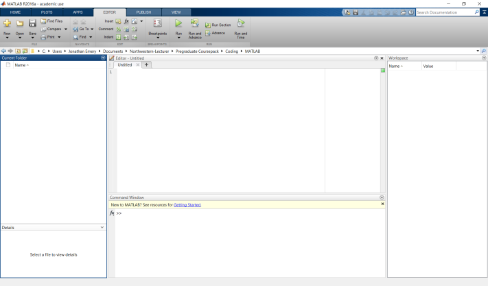
The MATLAB user interface, MATLAB 9.1.
This window (at the far left) shows the files that are present in your current directory. This can be changed by navigating to a different directory, shown in the field directly above the windows.
This window allows you to directly input commands in a command-line format. This is useful for simple, quick calculations and plots. For more extensive calculations you will need to write a script in the Editor.
You will use this space to write and edit your code. While you can, in principle, edit MATLAB code in any text editor, MATLAB’s editor is ideally suited to editing its own code and provides utilities that facilitate your scripting, including color-coded syntax, debugging options, and script comparison tools. These scripts are saved as so-called “m-files”, with extension
.m.The workspace contains data structures (scalars, vectors, matrices, tensors, and structure/cell arrays) that are created during your session. The woskpace provides you with at-a-glance information about, for example the data name, value, class, size, and statistics. You can view the data values by double-clicking on the data icon. This will open a sub-tab within the editor window which allows you to easily access and edit your data.
4.1.2 Basic Commands and Arithmetic Syntax
MATLAB possess its own scripting language and possess unique syntax. Below we list a selection — and some examples — of the most basic MATLAB commands. When appropriate, you can copy these examples directly into the command line or m-file and execute. The output will appear in the Command Window. This list is sourced from a document compiled from the \(\Eta \Kappa \Nu\) society at the University of Minnesota. The full source can be found here.
When operating in the command window there are a useful set of session managing commands that will streamline your workflow. These are listed in Tab. 1.
| Description | Syntax | Example |
|---|---|---|
| Session Management Operations | ||
| Clear command window | clc |
|
| Clear variables | clear |
|
| Returns help page | help |
help circshift |
| Set global variable | global |
global x |
| Quit MATLAB | quit |
|
| Display/use most resent answer | ans |
ans+2 |
Simple arithmetic operations and special variables are tabulated in Fig. 2.
| Description | Syntax | Example |
|---|---|---|
| Arithmetic Operations and Special Variables | ||
| Addition | + |
1+1 |
| Subtraction | - |
1-1 |
| Multiplication | * |
2*1 |
| Right-Hand Division | / |
1/2 |
| Left-Hand Division | ||
| ! | ||
| 2! | ||
| Exponentiation | ^ |
e^2 |
| Assignment | = |
a = 1 |
| Grouping | ( ) |
2*(3+6) |
| The number \(\pi\) | pi |
2*pi |
| Imaginary number \(\sqrt{-1}\) | i,j |
1 + 3i |
| Infinity | Inf |
1/0 |
| Not-a-Number | NaN |
Inf/Inf |
4.1.3 Matrix Notation and Operations
MATLAB is recognized for its strength in writing, representing, and operating on arrays. The construction of matrices in MATLAB is straightforward — examples are shown in Tab. 3.
When entering the example commands in the command line, a matrix-form output will be created. You can also see and edit these matrices by using the Workspace and accessing the Variable Spreadsheet.
| Description | Syntax | Example |
|---|---|---|
| Array Creation | ||
| Row Vector | [. . .] |
a = [1 2 3 4] |
| Column Vector | [. ; . ; .] |
a = [1; 2; 3; 4] |
| 2 \(\times\) 2 Matrix | [. . ; . . ;] |
a = [1 2; 3 4] |
| Create \(n \times m\) matrix | ||
ones(n,m) |
||
randi([-b,b],n,m) |
||
ones(3,5) |
||
rand([-5,5],4,4) |
||
| Accessing Matrix Elements | ||
| Access Row \(i\), column \(j\) of \(A\) | A(i,j) |
A(3,2) |
| Access \(i\)th row of \(A\) | A(i,:) |
A(1,:) |
| Access \(j\)th column of \(A\) | A(:,j) |
A(:,2) |
| Access submatrix of \(A\) | A([i1 i2],[j1, j2 ,3]) |
A([1 2], [1 2 4]) |
| Matrix Operations | ||
| Matrix Transpose | A' |
|
| Matrix Inverse | inv(A) |
|
| Matrix Multiplication | A*B |
|
| Matrix Inverse Multiplication | A/B or A*inv(B) |
|
| Matrix Exponentiation to \(n\) | A^n |
|
| Matrix Cross-product | cross(A,B) |
|
Matrix Dot-product dot(A,B) |
||
| Element-by-element operations | ||
A./B |
||
A.^n |
||
| Return \(n \times m\) size of A | size(A) |
|
| Concatenate column X onto A | [A X] |
|
| Concatenate row Y onto A | [A; Y] |
4.1.4 Creating and Using Functions
MATLAB has a large number of built-in function that can provided with input and provide an output. Simple examples include cos(x) or sqrt(x). When functions are called from script files they must be saved as individual files within the working directory (or a directory which has been added to the path). Example syntax for defining a “Power” function, which takes a input variable and outputs the computed result is shown below. This function can be called within a script to return variable p. The syntax here is: function [out1,out2, ..., outN] = myfun(in1,in2,in3, ..., inN), where in1 ... inN are input variables and out1, ..., outN are output variables.
Autonomous functions are another way to define a user-supplied function without necessitating the creation of a new file when calling them in a script. These can be defined in the command line or in-line within the m-file. An example of use of an autonomous function is shown in Fig. 0.1.7.
%% Power Function
% This function calculates x to the nth power.
% Returns variable p.

function [p] = Power(x,n)

p = x.^n;

end
4.1.5 Control Flow and Iterative Loops
A core component of any numerical calculation is the iterative loop that controls the simulation steps. These statements direct MATLAB to perform a certain calculation either while certain conditions are true or for certain a specific range/specific number of times. The general syntax here is disp
for index = values
   statements
end
Below, we show an example of a for loop that simply displays the values over each iteration — here from -2 (start) to 4 (finish) in steps of 0.5 (del). In place of the disp command you can place any command or series of commands, of course.
%% Define variables and preallocate.
start = -2;                          %Beginning of range .
finish = 4;                          %End of range
del = 0.5;                           %Interval
A = zeros (( finish-start )/del ,1); %Preallocated column vector , defined by range and interval .
index = 1; %Starting index forvector A.

%% For loop and define vector elements
for n = start : del : finish %Range from start to finish with interval del
    index = index + 1; %Step index
    A(index ,1) = n; %Define element
end

disp (A);
A while loop is shown below. This statement is useful when you are unsure about when the condition may become untrue (e.g. convergence criteria, etc.). The same example as shown above is show below, but now for the case which the index is less than or equal to the number of elements in the matrix. This job is more suitable for a for loop, but we show it below using a while loop for comparison.
%% Define variables and preallocate.
n = -2;                          %Beginning of range.
finish = 4;                      %End of range
del = 0.5;                       %Interval
A = zeros((finish-n)/del,1);     %Preallocated column vector, defined by range and interval.
index = 1;                       %Starting index for vector A.

%% For loop and define vector elements
while index <= length(A(:,1))    %Condition for calculation
   n = n + del;
   A(index,1) = n;               %Define element
   index = index + 1;            %Step index
end

disp(A);                         %Display A in command window.
4.1.6 Basic Plotting
You will inevitably want to visualize your data or computational results. MATLAB has a variety of tools to facility this. There are many, many options to plot data. Below we show a simple 2D plot that has some plotting options defined including axis ranges and labels.
The plot command mesh renders a wireframe figure of a scaled \(sinc\) function with \(Z\) values plotted with color. Thre sult is shown in Fig. 2 \(X\) and \(Y\) values are vectors that describe the plane. The example below shows a full, annotated m-file in which the last section (the plot section) defines plotting options including axis for axis range and xlabel for axis labels.
%% MeshPlot.m
% A simple script with an anonymous function to plot a radial sinc function.
% Author: JD Emery
% Modified: Feb 18th 2017

%% Variable Declaration/Preallocation
a = 2;
b = 3;

%% Anonymous Functions
sinc2 = @(x,y) x*sin(y)./y;   %Define anonymous function sinc2 with inputs (x,y)

%% Script
[X,Y] = meshgrid(-20:.25:20); %Define the mesh calculation range.
R = sqrt(a*X.^2 + b*Y.^2);    %Define value R in terms of X,Y meshpoints.

%% Plot
f = figure; %Create figure and define handle.
set(f,'name','Sinc Function 2D','numbertitle','off') %Name figure

mesh(X,Y,sinc2(a,R),'LineWidth',0.3) %Plot [X,Y,Z] using mesh tool.
axis([-8 8 -8 8 -1 2]) %Set plotranges
xlabel('-8 < x < 8') % x-axis label
ylabel('-8 < y < 8') % y-axis label
zlabel('sinc(x*R)')  %z-axis label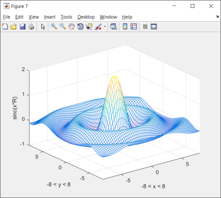
A meshplot of a sinc function.
4.1.7 Scripting and Debugging the m-file
Working with the command line is convenient for quickly accessing and working with data, or running scripts or creating custom functions. The examples above can be simply executed line-by-line in the the command window (although they were written as m-files), in doing so you will soon find, however, that it is much more convenient to write a script — a series of commands — in a m-file within the MATLAB editor. A script m-file operates simply by executing any commands listed in the file. A somewhat more advanced example is shown in Section 0.1.6. A very simple example for an m-file that uses the disp command to print “Hello World”in the command window is shown below.
The example below also contains a commented-out % preamble with file information as well as section breaks %% for organization.
%% HelloWorld.m
% A simple script for "Hello World"
% Author: JD Emery
% Modified: Feb 18th 2017

%%
disp('Hello World')
Script m-files usually possess at least four sections (examples of all these sections, as well as a plotting section are shown in 0.1.6):
This is where you will record pertinent notes about the file such as version history, authorship, licensing, or other comments. These are usually commented out with % symbols.
After the preamble there is typically a section where you define the variables that will be used in the script5. Preallocation of arrays with
zeros(n,m)orones(n,m)can greatly reduce the amount of memory consumed by MATLAB — especially when arrays iteratively grow when the script is run.Often, you will want to add a function that is not built into MATLAB syntax or that does not need its own program file. These functions are often added at the end the m-file and are accessed when the script is run.
This is where the calculations are performed and the data is saved or plotted.
MATLAB provides a number of interactive tools to simplify coding and debugging. Useful tools exist in the editor ribbon, including insert of sections of functions (from a library) or indent and comment control. Arguably, the most valuable tool is the setting and handling of breakpoints. Breakpoints are especially useful when constructing loops because the calculations can be monitored step-by-step through the loop.
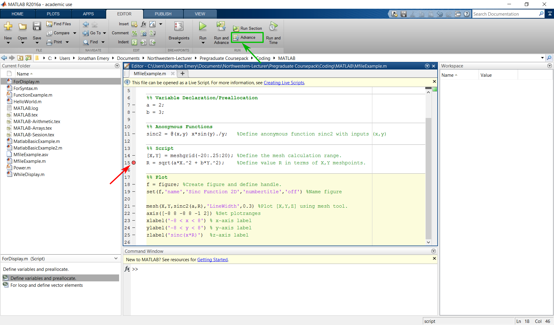
Debugging MATLAB scripts.
To set a breakpoint simply left click on the horizontal dash next to the line you would like to break at (indicated with a red arrow, Fig. 3). Run the code. Your script will stop at this point and you can investigate variable values. Then, you can advance the code to the next breakpoint (Fig. 3, green square). When in a loop this command will iterate the loop one step. When ready, you can use the breakpoints button to eliminate all breakpoints and run the code.
4.2 Mathematica (Release TBD)
Mathematica is useful for symbolic mathematical computation. It is free for all students.
4.2.1 Suggested Resources:
The Wolfram Language: Fast Introduction for Programmers,
Symbolic and Numeric Representations and Calculations
Basic Plotting: 2D, 3D and interactive
Linear Algebra: Matrix Operations and Notations
Equation Solvers (\(\rightarrow\) step-by-step solutions with WolframAlpha access).